원본 링크

Dimensionality Reduction — Can PCA improve the performance of a classification model?

PCA를 사용한 ML 모델 성능 개선 - 차원감소 기술

Photo by Olav Ahrens Røtne on Unsplash

What is PCA?

중요요소분석(Principal Component Analysis, PCA)은 데이터 과학에서 더 낮은 공간으로 데이터의 차원을 감소시키기 위해 행렬 인수분해(matrix factorization)를 사용하는 일반적인 특성 추출 기술이다.

실제 데이터셋에서는 종종 데이터에 너무 많은 특성이 있다. 더 많은 특성의 수는 데이터를 시각화하고 작업하기 더 힘들다. 때때로 특성의 대부분이 관계되어 있기 때문에 불필요하다. 그래서 특성 추출을 적용하기 시작한다.

About the Data:

이 글에서는 Ionosphere Dataset from the UCI machine learning repository의 이진분류 데이터셋을 사용한다. 이 데이터셋은 34개의 특성을 가진 351개의 데이터이다.

Preparing the Dataset:

• 필요한 라이브러리를 import하고 데이터셋을 읽는다.
• 데이터셋을 전처리한다.
• 표준화(Standardization)한다.

  
  import pandas as pd
  import numpy as np
  from sklearn.preprocessing import StandardScaler
  rom sklearn.model_selection import train_test_split
  
  

y_train = y_train.astype('int')
y_test = y_test.astype('int')


Logistic Regression ML model using all 34 features:

훈련 데이터는 34개의 특성이 있다.

• 데이터 전처리후 훈련데이터는 이진분류를 위한 Logistic Regression 알고리즘을 사용하여 훈련된다.

• 최고의 파라미터를 찾기 위해 Logistic Regression 모델을 세부조정(finetune)한다.

• 훈련 및 테스트 정확도, f1-점수를 계산한다.
  

  
  (Image by Author), Plot of C vs F1 score for the logistic regression model for 34 features dataset
  

• $c=10^x$에 대한 34가지 특성을 사용하여 모델을 훈련한다.

• 훈련과 테스트 그리고 f1 점수를 계산한다.
  

  
  (Image by Author), Train-Test accuracy and F1-score, Confusion Matrix
  

34 개의 특성을 가진 전체 "X_train"데이터를 훈련하여 얻은 결과,

Confusion matrix에서 관측된것과 같이 14개의 미분류 값이 있기 때문에 test f1-점수는 0.90이다.

import matplotlib.pyplot as plt
from sklearn.linear_model import LogisticRegression
from sklearn.metrics import *

C = [10**-3, 10**-2, 10**-1, 10**0, 10**1, 10**2, 10**3, 10**4]
f1_tr = []
f1_te = []
for c in C:
    model = LogisticRegression(C=c)
    model.fit(X_train_std, y_train)
    f1_te.append(f1_score(model.predict(X_test_std), y_test))
    f1_tr.append(f1_score(model.predict(X_train_std), y_train))
    print(c, f1_score(model.predict(X_test_std), y_test))

plt.plot(C, f1_te, label="Test")
plt.plot(C, f1_tr, label="Train")
plt.xlabel("Hyperparameter C")
plt.ylabel("F1 score")
plt.xscale("log")
plt.legend()
plt.grid()
plt.show()

model = LogisticRegression(C=10**0)
model.fit(X_train_std, y_train)

y_pred_te = model.predict(X_test_std)
y_pred_tr = model.predict(X_train_std)

print("Test acc", accuracy_score(y_test, y_pred_te))
print("Train acc", accuracy_score(y_train, y_pred_tr))

print("Test f1", f1_score(y_test, y_pred_te))
print("Train f1", f1_score(y_train, y_pred_tr))

print(confusion_matrix(y_test, y_pred_te))

Feature Extraction using PCA:

PCA 기술을 사용하여 데이터셋에서 특성을 추출하려면 우선 차원이 감소(dimensionality decreases)하는 것으로 설명되는 분산(variance)의 비율(percentage)을 알아야 한다.

• $\lambda$ : 고유값(eigenvalue)
• $d$ : 원본 데이터셋 차원수(number of dimension)
• $k$ : 새로운 특성 공간의 차원수
  

(Image by Author), Plot for % of variance explained vs the number of dimensions

• 위 그래프에서 15차원에 대해 설명되는 분산의 비율은 90%인 것을 볼 수 있다. 이는 더 높은 차원(34차원)을 더 낮은 공간(15차원)으로 투영하여 90%의 분산을 보존하고 있다는 의미이다.
  

  
  from sklearn.decomposition import PCA
  
  

pca = PCA(n_components=15)
pca_train_data = pca.fit_transform(X_train_std)
pca_test_data = pca.transform(X_test_std)


Training Logistic Regression ML model using top 15 features from PCA:

이제 PCA 차원감소 후 훈련 데이터는 15개의 특성을 갖는다.

• 데이터의 전처리후 훈련데이터는 이진 분류를 위한 Linear Regression 모델 훈련에 사용된다.

• 최고의 파라미터를 찾기 위해 모델을 세부튜닝한다.

• 훈련과 테스트 그리고 f1 점수를 계산한다.
  

  
  (Image by Author), Plot of C vs F1 score for the logistic regression model for 15 features dataset
  

• $c=10^x$에 대한 15가지 특성을 사용하여 모델을 훈련한다.

• 훈련과 테스트 그리고 f1점수를 계산한다.
  

  
  (Image by Author), Train-Test accuracy and F1-score, Confusion Matrix
  

15가지 특성으로 PCA 데이터를 훈련하여 얻은 결과,
Confusion matrix에서 관측된 것과 같이 12개의 미분류값이 있기 때문에 test f1점수는 0.896이다.

Comparing the results of the above two models:

(Image by Author), Train-Test accuracy and F1-score, Confusion Matrix

import matplotlib.pyplot as plt
from sklearn.linear_model import LogisticRegression
from sklearn.metrics import *

C = [10**-3, 10**-2, 10**-1, 10**0, 10**1, 10**2, 10**3, 10**4]
f1_tr = []
f1_te = []
for c in C:
    model = LogisticRegression(C=c)
    model.fit(X_train_std, y_train)
    f1_te.append(f1_score(model.predict(X_test_std), y_test))
    f1_tr.append(f1_score(model.predict(X_train_std), y_train))
    print(c, f1_score(model.predict(X_test_std), y_test))

plt.plot(C, f1_te, label="Test")
plt.plot(C, f1_tr, label="Train")
plt.xlabel("Hyperparameter C")
plt.ylabel("F1 score")
plt.xscale("log")
plt.legend()
plt.grid()
plt.show()

model = LogisticRegression(C=10**0)
model.fit(X_train_std, y_train)

y_pred_te = model.predict(X_test_std)
y_pred_tr = model.predict(X_train_std)

print("Test acc", accuracy_score(y_test, y_pred_te))
print("Train acc", accuracy_score(y_train, y_pred_tr))

print("Test f1", f1_score(y_test, y_pred_te))
print("Train f1", f1_score(y_train, y_pred_tr))

print(confusion_matrix(y_test, y_pred_te))

Training LR model using original data + data from PCA:

34가지 특성을 가진 원본 데이터와 15가지 특성을 가진 PCA 데이터를 합쳐 49가지 특성을 가진 데이터셋을 만든다.

• 데이터 전처리 후 이진 분류를 위해 Logistic Regression 알고리즘을 사용하여 훈련한다.

• 최고의 파라미터를 찾기 위해 모델을 세부튜닝한다.

• 훈련과 테스트 그리고 f1 점수를 계산한다.
  

  
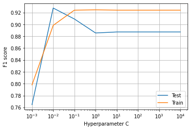
  (Image by Author), Plot of C vs F1 score for the logistic regression model for 49 features dataset
  

• $c=10^x$에 대한 15가지 특성을 사용하여 모델을 훈련한다

• 훈련과 테스트 그리고 f1 점수를 게산한다.
  

  
  (Image by Author), Train-Test accuracy and F1-score, Confusion Matrix
  

  
  concat_train_data = np.concatenate((X_train_std, pca_train_data), 1)
  concat_test_data = np.concatenate((X_test_std, pca_test_data), 1)
  
  

print(confusion_matrix(y_test, y_pred_te))


Conclusions from the above results:

(Image by Author), Accuracy and F1-score results for the above three models

위 표에서 다음을 알 수 있다.

• 34가지 특성을 가진 원본 전처리된 데이터셋을 사용한 모델로 90%의 f1점수를 얻었다.
• PCA를 사용하여 15가지 특성이 추출된 것으로만 훈련한 모델로는 89%의 f1점수를 얻었다.
• 위 두 데이터를 조합하여 훈련한 모델로는 92%의 f1점수를 얻었다.
  

위에서 언급된 3가지 모델에 대한 confusion matrix에서 변화를 찾아보자.

(Image by Author), Confusion Matrix for the above three models

따라서 원본 데이터에서 50%의 특성수만을 갖는 PCA로 추출된 특성만을 사용하여 1% 적은 f1 점수를 얻는다고 할 수 있고 두 데이터를 조합하면 최종 91%의 f1점수를 얻는 2%의 지표(metric)를 개선한다.